
We are thrilled to share that the
palmerpenguins package is now available on
CRAN! 
The palmerpenguins R package contains two datasets that we believe are a viable alternative to Anderson’s Iris data (via
datasets::iris). And just in time for fall, the penguins have landed on CRAN 🎉 They are pretty excited about this (as you can tell). Now, it will be easier for you and your students to get to know them. We also hope it makes it easier for educators and software developers to
move on from iris. Here is just one example, plotting the lengths of penguin flippers versus their bills:

You can install the released version of palmerpenguins from CRAN with:
install.packages("palmerpenguins")
In this post, we’ll share some highlights that we think make palmerpenguins fun for teaching data science and statistics. We’ll use functions from the tidyverse to demonstrate:
library(tidyverse)
library(palmerpenguins)
Note: these are not Antarctic penguins; these are Magellanic penguins from the Monterey Bay Aquarium 🐧 But we love them anyway. And these South African penguins want to see what all the fuss about too.
Meet the penguins
The palmerpenguins data contains size measurements, clutch observations, and blood isotope ratios for three penguin species observed on three islands in the Palmer Archipelago, Antarctica over a study period of three years.

These data were collected from 2007 - 2009 by Dr. Kristen Gorman with the Palmer Station Long Term Ecological Research Program, part of the US Long Term Ecological Research Network. The data were imported directly from the Environmental Data Initiative (EDI) Data Portal, and are available for use by CC0 license (“No Rights Reserved”) in accordance with the Palmer Station Data Policy. We gratefully acknowledge Palmer Station LTER and the US LTER Network. Special thanks to Marty Downs (Director, LTER Network Office) for help regarding the data license & use. Here is our intrepid package co-author, Dr. Gorman, in action collecting some penguin data:

You can find this photo and others in a shared Google slideshow, meant to help you teach with this data.
Here is a map of the study site:

The palmerpenguins package
This package contains two datasets:
-
The raw data is available as
penguins_raw. -
A curated subset of the raw data in the package named
penguins, which can serve as an out-of-the-box alternative todatasets::iris.
When you first call either of these datasets, what you see depends on whether or not you have the
tibble package installed on your local workstation. If you do have the tibble package installed, then you will see the first 10 rows of data print as a nice tidy tibble. If not, you’ll see the full dataset print to your console, just as iris does. This allowed us to keep palmerpenguins as lightweight as possible for all users, and yet still user-friendly for tidyverse beginners. A big thank you to Hadley Wickham for contributing this
creative solution!
The curated palmerpenguins::penguins dataset contains 8 variables (n = 344 penguins). You can read more about the variables by typing ?penguins.
penguins
#> # A tibble: 344 x 8
#>    species island bill_length_mm bill_depth_mm flipper_length_… body_mass_g
#>    <fct>   <fct>           <dbl>         <dbl>            <int>       <int>
#>  1 Adelie  Torge…           39.1          18.7              181        3750
#>  2 Adelie  Torge…           39.5          17.4              186        3800
#>  3 Adelie  Torge…           40.3          18                195        3250
#>  4 Adelie  Torge…           NA            NA                 NA          NA
#>  5 Adelie  Torge…           36.7          19.3              193        3450
#>  6 Adelie  Torge…           39.3          20.6              190        3650
#>  7 Adelie  Torge…           38.9          17.8              181        3625
#>  8 Adelie  Torge…           39.2          19.6              195        4675
#>  9 Adelie  Torge…           34.1          18.1              193        3475
#> 10 Adelie  Torge…           42            20.2              190        4250
#> # … with 334 more rows, and 2 more variables: sex <fct>, year <int>
Highlights
We don’t want to ruin all the fun exploration, visualization, and potential analyses, so below are just a few examples to get you quickly waddling along with penguins. You can check out more in the “Get started” and the “Examples” vignettes.

If you are teaching correlation and simple linear regression, penguin flipper length and body mass show a positive association for each of the 3 species:
# Scatterplot example 1: penguin flipper length versus body mass
ggplot(data = penguins, aes(x = flipper_length_mm, y = body_mass_g)) +
  geom_point(aes(color = species,
                 shape = species),
             size = 2) +
  scale_color_manual(values = c("darkorange","darkorchid","cyan4"))

Penguin bill length and depth also show some interesting patterns. If you ignore species, you might think there is a negative correlation:
# Scatterplot example 2: penguin bill length versus bill depth
ggplot(data = penguins, aes(x = bill_length_mm, y = bill_depth_mm)) +
  geom_point(size = 2) +
  geom_smooth(method = "lm", se = FALSE)

But, if you look at the correlations within species, bill length and depth are actually positive correlated. This is a nice “in the wild” example of Simpson’s paradox.
# Scatterplot example 3: penguin bill length versus bill depth
ggplot(data = penguins, aes(x = bill_length_mm, y = bill_depth_mm)) +
  geom_point(aes(color = species,
                 shape = species),
             size = 2) +
  geom_smooth(method = "lm", se = FALSE, aes(color = species)) +
  scale_color_manual(values = c("darkorange","darkorchid","cyan4"))

At this point, you may be also want to know how bill length and depth were actually measured. Luckily, Allison Horst drew up some illustrations to help explain this. Here is one for bill measurement:

You can download this and other palmerpenguins art (useful for teaching with the data) directly from the package website. If you use this artwork, please cite with: “Artwork by @allison_horst".
Finally, you can get a pretty clear separation between all three species by looking at flipper length versus bill length:
ggplot(penguins, aes(x = flipper_length_mm, y = bill_length_mm, colour = species, shape = species)) +
  geom_point() +
  scale_colour_manual(values = c("darkorange","purple","cyan4"))

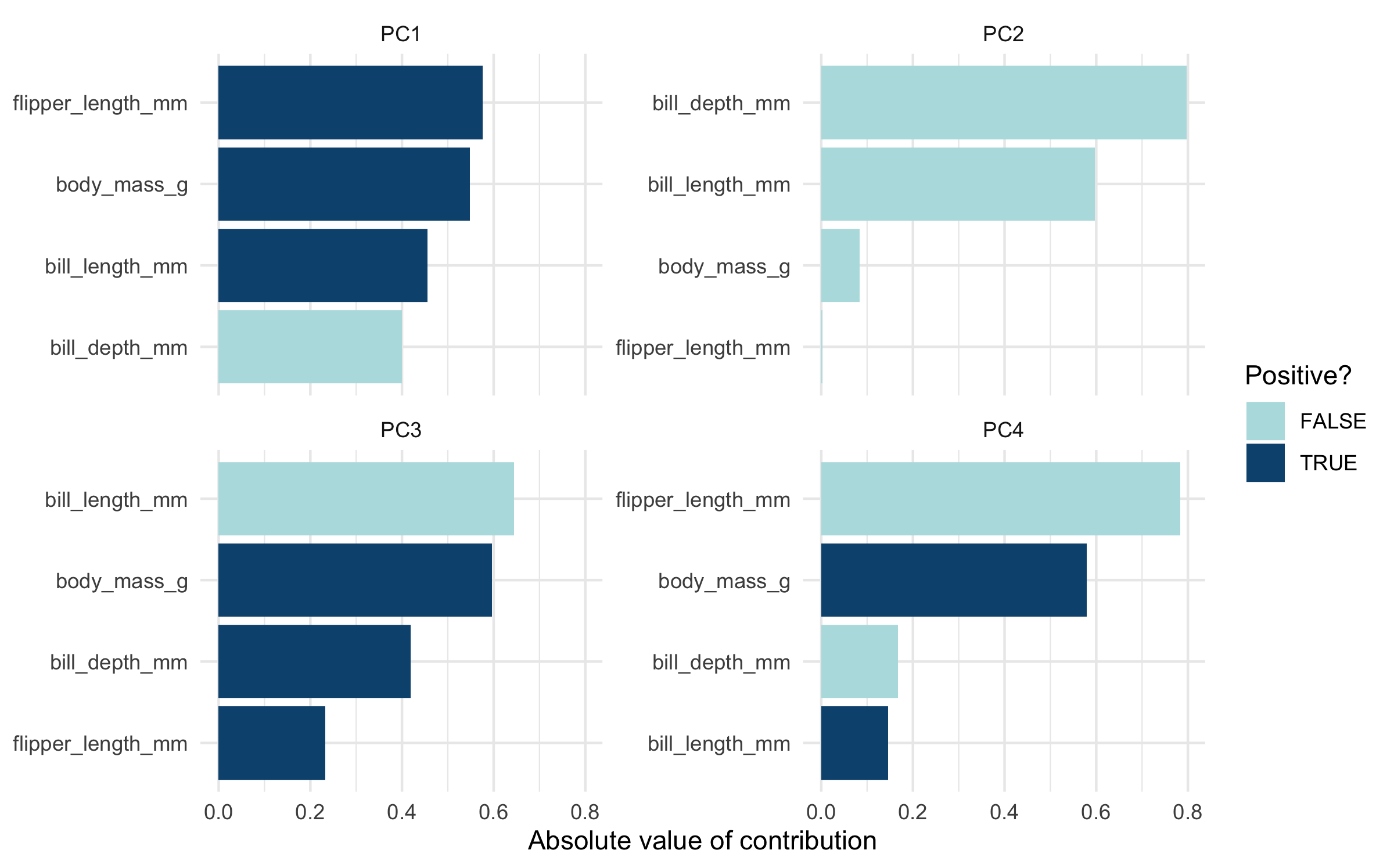
This ends up leading to some nice results using principal components analysis, which is commonly done with iris as a “hello world” PCA example. We provide code to do a simple PCA using
tidymodels in the
“PCA with penguins and recipes” vignette.
We are also pleased to report that the penguins enjoy clustering as well. Here is an example using K-means clustering with two tidymodels packages, broom and recipes.

One more thing! If you want to give your students experience importing and wrangling data, we made a function that allows you to access the .csv files from within the package. Here is an example of how you use it:
raw_csv <- readr::read_csv(path_to_file("penguins_raw.csv"))
raw_csv
#> # A tibble: 344 x 17
#>    studyName `Sample Number` Species Region Island Stage `Individual ID`
#>    <chr>               <dbl> <chr>   <chr>  <chr>  <chr> <chr>
#>  1 PAL0708                 1 Adelie… Anvers Torge… Adul… N1A1
#>  2 PAL0708                 2 Adelie… Anvers Torge… Adul… N1A2
#>  3 PAL0708                 3 Adelie… Anvers Torge… Adul… N2A1
#>  4 PAL0708                 4 Adelie… Anvers Torge… Adul… N2A2
#>  5 PAL0708                 5 Adelie… Anvers Torge… Adul… N3A1
#>  6 PAL0708                 6 Adelie… Anvers Torge… Adul… N3A2
#>  7 PAL0708                 7 Adelie… Anvers Torge… Adul… N4A1
#>  8 PAL0708                 8 Adelie… Anvers Torge… Adul… N4A2
#>  9 PAL0708                 9 Adelie… Anvers Torge… Adul… N5A1
#> 10 PAL0708                10 Adelie… Anvers Torge… Adul… N5A2
#> # … with 334 more rows, and 10 more variables: `Clutch Completion` <chr>, `Date
#> #   Egg` <date>, `Culmen Length (mm)` <dbl>, `Culmen Depth (mm)` <dbl>,
#> #   `Flipper Length (mm)` <dbl>, `Body Mass (g)` <dbl>, Sex <chr>, `Delta 15 N
#> #   (o/oo)` <dbl>, `Delta 13 C (o/oo)` <dbl>, Comments <chr>
You can see the files available by using the path_to_file() function without any arguments:
path_to_file()
#> [1] "penguins_raw.csv" "penguins.csv"
Credit goes to Jenny Bryan for this function, inspired by a similar function in the readxl package.
And as a reminder, you can always read the data in from a url as well:
peng_url <- readr::read_csv("https://raw.githubusercontent.com/allisonhorst/palmerpenguins/master/inst/extdata/penguins.csv")
peng_url
#> # A tibble: 344 x 8
#>    species island bill_length_mm bill_depth_mm flipper_length_… body_mass_g
#>    <chr>   <chr>           <dbl>         <dbl>            <dbl>       <dbl>
#>  1 Adelie  Torge…           39.1          18.7              181        3750
#>  2 Adelie  Torge…           39.5          17.4              186        3800
#>  3 Adelie  Torge…           40.3          18                195        3250
#>  4 Adelie  Torge…           NA            NA                 NA          NA
#>  5 Adelie  Torge…           36.7          19.3              193        3450
#>  6 Adelie  Torge…           39.3          20.6              190        3650
#>  7 Adelie  Torge…           38.9          17.8              181        3625
#>  8 Adelie  Torge…           39.2          19.6              195        4675
#>  9 Adelie  Torge…           34.1          18.1              193        3475
#> 10 Adelie  Torge…           42            20.2              190        4250
#> # … with 334 more rows, and 2 more variables: sex <chr>, year <dbl>
The .csv files are located in the
package GitHub repository in the
inst/extdata/ folder.
Penguin sightings
You can access the palmerpenguins data outside of R too! Our sincere thanks to all the contributors who made the penguins popular. Here are some other places you might spot the palmerpenguins:
Python
Python users can access the penguins data in the seaborn data visualization library. Example code to load the data in Python:
import seaborn as sns
df = sns.load_dataset(‘penguins’)
Julia
Julia users can access the penguins data in the PalmerPenguins.jl package. Example code to import the penguins data through PalmerPenguins.jl:
julia> using PalmerPenguins
julia> table = PalmerPenguins.load()
OpenML
openml.org is a public repository for machine learning data and experiments. Find the penguins here:
https://www.openml.org/d/42585
You can also download the penguins from the openml.org repository with Python using scikit-learn:
from sklearn.datasets import fetch_openml
penguins = fetch_openml(name='penguins', version=1)
Tidy Tuesday
The penguins are chuffed to be the dataset this week! Check out the announcement here: https://github.com/rfordatascience/tidytuesday/blob/master/data/2020/2020-07-28/readme.md
Kaggle
https://www.kaggle.com/parulpandey/palmer-archipelago-antarctica-penguin-data
Makeover Monday
Makeover Monday featured the penguins on 2020/07/13.
Meetups & talks
Here are recent highlights on our penguin radar!
-
Di Cook: Going beyond 2D and 3D to visualise higher dimensions, for ordination, clustering and other models

-
Samantha Toet: Building dashboards with flexdashboard and Shiny

Contribute your own examples
If you use palmerpenguins, please consider sharing with us and add it to our user-contributed examples. And don’t forget about the photos and art to help you teach with the palmerpenguins!
Penguin citation
Please cite the palmerpenguins R package using:
citation("palmerpenguins")
#>
#> To cite palmerpenguins in publications use:
#>
#>   Horst AM, Hill AP, Gorman KB (2020). palmerpenguins: Palmer
#>   Archipelago (Antarctica) penguin data. R package version 0.1.0.
#>   https://allisonhorst.github.io/palmerpenguins/. doi:
#>   10.5281/zenodo.3960218.
#>
#> A BibTeX entry for LaTeX users is
#>
#>   @Manual{,
#>     title = {palmerpenguins: Palmer Archipelago (Antarctica) penguin data},
#>     author = {Allison Marie Horst and Alison Presmanes Hill and Kristen B Gorman},
#>     year = {2020},
#>     note = {R package version 0.1.0},
#>     doi = {10.5281/zenodo.3960218},
#>     url = {https://allisonhorst.github.io/palmerpenguins/},
#>   }
Have fun with the Palmer Archipelago penguins!
References
Data originally published in:
- Gorman KB, Williams TD, Fraser WR (2014). Ecological sexual dimorphism and environmental variability within a community of Antarctic penguins (genus Pygoscelis). PLoS ONE 9(3):e90081. https://doi.org/10.1371/journal.pone.0090081
Individual datasets:
Individual data can be accessed directly via the Environmental Data Initiative:
-
Palmer Station Antarctica LTER and K. Gorman, 2020. Structural size measurements and isotopic signatures of foraging among adult male and female Adélie penguins (Pygoscelis adeliae) nesting along the Palmer Archipelago near Palmer Station, 2007-2009 ver 5. Environmental Data Initiative. https://doi.org/10.6073/pasta/98b16d7d563f265cb52372c8ca99e60f (Accessed 2020-06-08).
-
Palmer Station Antarctica LTER and K. Gorman, 2020. Structural size measurements and isotopic signatures of foraging among adult male and female Gentoo penguin (Pygoscelis papua) nesting along the Palmer Archipelago near Palmer Station, 2007-2009 ver 5. Environmental Data Initiative. https://doi.org/10.6073/pasta/7fca67fb28d56ee2ffa3d9370ebda689 (Accessed 2020-06-08).
-
Palmer Station Antarctica LTER and K. Gorman, 2020. Structural size measurements and isotopic signatures of foraging among adult male and female Chinstrap penguin (Pygoscelis antarcticus) nesting along the Palmer Archipelago near Palmer Station, 2007-2009 ver 6. Environmental Data Initiative. https://doi.org/10.6073/pasta/c14dfcfada8ea13a17536e73eb6fbe9e (Accessed 2020-06-08).
Acknowledgements
A big thank you to all palmerpenguins contributors: @allisonhorst, @amrrs, @apreshill, @brunj7, @devmotion, @eddelbuettel, @friendly, @hadley, @jannikbuhr, @jhk0530, @john-sandall, @karaesmen, @markvanderloo, @trang1618, and @ttimbers